Stochastic Gradient Descent and its variants, referred here collectively as SGD, have been the de facto methods in training neural networks. These methods aim to minimize a network-specific loss function F(x) whose lower values correspond to better-trained versions of the neural network in question. To find a minimal point x*, SGD relies solely on knowing the gradient (approximately) at the neural network weights xk at iteration k. Hence SGD is ▽F(xk) considered a first-order method as it uses only gradient and not curvature information about F(x).
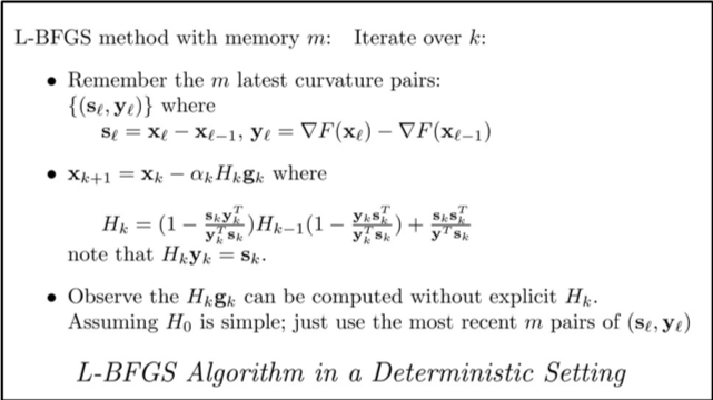
My collaborators Raghu Bollapragada, Jorge Nocedal, Hao-Jun Michael Shi from Northwestern University, and Dheevatsa Mudigere from Intel Labs in Bangalore, India have recently adapted the higher-order L-BFGS optimization method to a stochastics setting suitable for machine learning. We derived various convergence proofs of our algorithm, and its implementation exhibits encouraging experimental results. In this blog post, I will informally introduce the work, and the full paper can be found here.
Why Explore L-BFGS?
In optimization theory and practice, higher-order methods often outperform first-order methods significantly. Textbooks such as [1] routinely present examples where a higher-order algorithm requires two orders of magnitude fewer iterations to converge compared to a first-order analogue. Provided below are high-level descriptions of them. A first-order method tries to find a minimal point of F(x) moving x along the negative direction of the gradient: –▽F(x) as shown on the top part of the figure. That is, it uses information on how F(x) changes. A higher-order method tries to find a zero of F(x)’s gradient using information on how▽F(x) changes. Newton’s Method is the best-known higher-order method where x is moved along –(▽2F(x))-1▽F(x) which involves applying the inverse of the Hessian matrix to the gradient of F. In the context of machine learning, Newton’s Method is impractical as the cost of applying the inverse Hessian is exorbitant. A quasi-Newton method reduces the cost by approximating the Hessian—the gradient of▽F(x) —by a secant, H, of▽F(x). A matrix H is said to satisfy the secant condition corresponding to two points x and x' as long as H(▽F(x') – ▽F(x)) = x' – x. Given a current position x, a quasi-Newton method will move x along the direction of –H(▽F(x)).
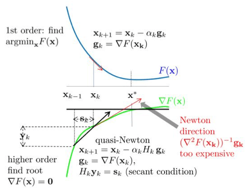
The limited memory version L-BFGS [2] relaxes the memory requirement by using only a fixed number (10 usually suffice) of the most recent curvature pairs. That it works even better in practice than its well-established convergence theory makes L-BFGS one of the favorite methods for standard (non-machine learning-specific) optimization problems.
How L-BFGS is Adapted
In training neural networks, however, deterministic approaches become infeasible. Typically, the function F(x) to be optimized is given as a sum with the number of summands equal to the size of the training set in question. A stochastic approach is taken where at each iteration, one only deals with a sample of these summands whose (stochastic) gradient we compute. The following notation is common:
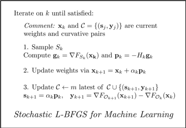
The underlying principle is to obtain a stochastic gradient such that not only the expected direction is applied to the exact gradient, but also that Ρk makes a small angle with the latter in high probability. We developed a simple estimate relating the variance of this angle to the batch size |Sk|. The batch size |Sk| is thus increased progressively to keep the variance within a threshold that is chosen as a hyperparameter.
Step Size αk via Stochastic Line Search
Long-established analysis for deterministic BFGS and L-BFGS suggests initializing αk <– 1 and repeatedly shrinking it (“backtracking” in optimization terminology) until the decrease seen in F(xk + αkΡk) is deemed acceptable. We extended that analysis to our stochastic setting and derived a starting value for αk in terms of various statistics involving▽F(xk) and Hkgk. We, therefore, initiate our line search based on this formula and estimates on the various quantities that it contains.
Computing Consistent Curvature Pairs
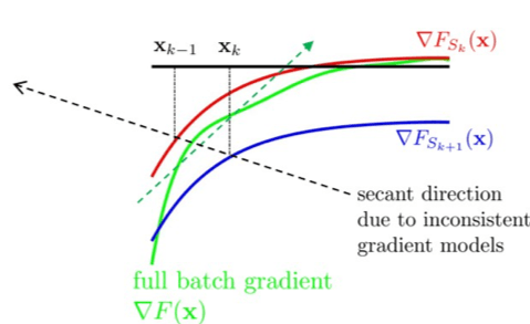
Note that the curvature pair (Sl, Yl) in the deterministic case involves the difference between two gradients: In Step 3, we need Yk+1 =▽F(xk+1) – ▽F(xk). In the machine learning setting, we can only practically afford to compute “approximate” gradients based on a stochastically chosen batch. Thus the formula looks like Yk+1 =▽FOk+1(xk+1) – ▽FOk(xk). The immediate question is: how should we choose the batches Ok+1 and Ok. The most convenient choice of Ok = Skand Ok+1 = Sk+1 (the latter is feasible as we note that Yk+1 is not really needed until Step 2 of the next iteration) is problematic as illustrated by the simple picture here: while both approximate gradients represent the trending of the correct gradient (green one), their differences can be unpredictable. We use two possible choices in our adaptation: the first is to use Ok+1 = Ok = Sk, called the fully overlapped mode. In the fully overlapped mode, consistency is maintained by doubling the cost of gradient evaluation as▽Fsk(xk+1) and is not needed anywhere else. To mitigate this cost, we also use an alternative method called multi-batchmode. Here we use a small subset (e.g. 25%) of Sk: Ok+1 = Ok ⊂ Sk) and make sure that the stochastic batch Sk+1 in the next iteration also contains this subset. Consequently, no extra cost of gradient evaluation is incurred at all. Our experiments show that both approaches work and thus multi-batch should be the default mode of operation.
Where We are at, and What the Next Steps are
Our paper establishes several convergence results such as linear convergence when the loss function is strongly convex, and general (slower) convergence without convexity assumptions. We apply our algorithm on a logistic regression problem on eight datasets and on several neural networks of convolutional and residual types on the MNIST and CIFAR-10 datasets. We present just a snapshot of these results here and invite our readers to read through our paper on the archive site.
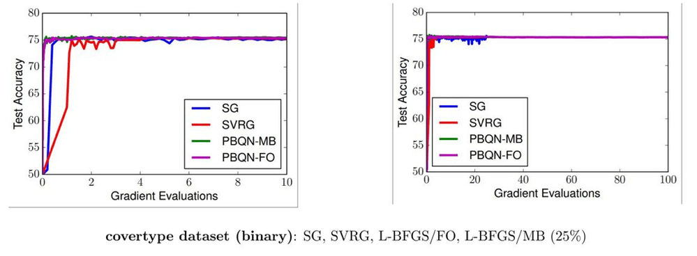
For the logistic regression problem, we compared with the standard SGD approach and also the variance reduction method of SVRG. The two figures below show the test accuracy versus number of (full) gradient evaluations, also called epochs. This shows that a higher-order method is highly competitive with other training methods, a concept not commonly shared as exhibited in Figure 3.1 of [3].
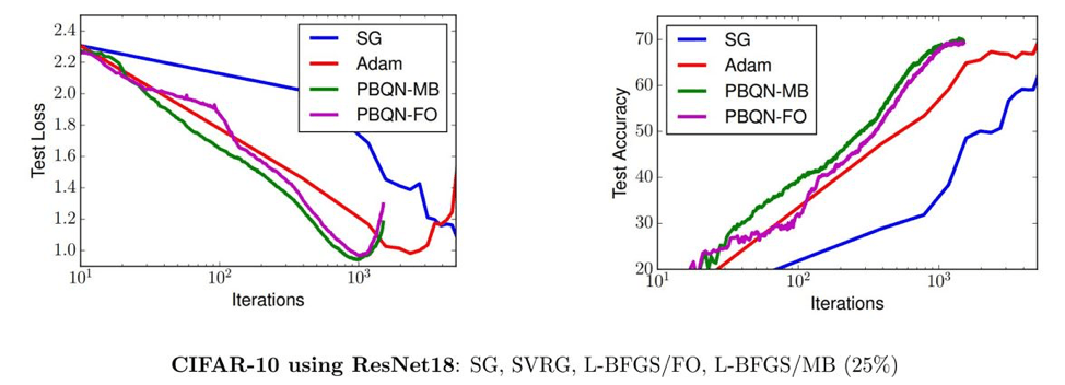
The figures below show that our progressive batching L-BFGS, while promising, requires more work on general neural networks. Compared with SGD and Adam, L-BFGS exhibits reasonable progress in test loss reduction until it overfits. We are currently working on several ideas to mitigate overfitting and a fully parallel implementation as a progressive increasing batch size is most amenable to massive parallelism.
References
[1] Nocedal, J. and Wright, S. Numerical Optimization. Springer New York, 2nd edition, 1999.
[2] Liu, D. C. and Nocedal, J. On the limited memory BFGS method for large scale optimization. Mathematical Programming, 45(1-3): 503-528, 1989.
[3] Bottou, L. Curtis, F. and Nocedal, J. Optimization methods for large-scale machine learning. SIAM Review, 60-2: 223-311, 2018.
 Mary is the Community Manager for this site. She likes to bike, and do college and career coaching for high school students in her spare time.
You must be a registered user to add a comment. If you've already registered, sign in. Otherwise, register and sign in.

