Optimizing Graph Neural Network Training Performance on Intel® Xeon®

Published February 9th, 2022

Sasikanth Avancha is a research scientist at Intel Labs working toward the next generation of high-performance machine learning software and hardware architectures.

Over the past several years, Deep Learning (DL) techniques have transformed applications such as computer vision and natural language processing. Typically, these applications operate on data defined over a 2-dimensional grid, 3-dimensional volume, or other structures over n-dimensional Euclidean space. However, popular DL techniques, such as Convolutional Neural Network (CNN) or Multi-Layer Perceptron (MLP) models are insufficient to capture the structure of data in non-Euclidean space. Graphs are an example of a data structure that captures relationships between data elements in non-Euclidean domains. Well-known examples of graphs in the real world are the Internet, social networks, web-scale networks, biomedical networks, and economic networks. Traditional approaches to discovering the structure of data in such networks involve algorithms such as breadth-first search (BFS), depth-first search (DFS), triangle counting, connected components, etc., which in combination refer to the computer science domain of graph analytics. 

Graph Neural Networks (GNN) is a modern, data-driven approach to analyzing large graphs and discovering their structure. A GNN consists of three key components: (i) information associated with each node (and optionally each edge) in the graph, represented as a single-dimensional vector known as an embedding, (ii) a recursive message-passing aggregation algorithm that aggregates vertex/edge embeddings in novel ways and (iii) a neural network model (typically an MLP), that learnsthe graph structure iteratively via standard gradient-descent training algorithms used in DL. The impact of GNNs on the modern world cannot be overstated – they have the power to analyze complex relationships at both the macro scale such as the Internet or social media networks and the micro-scale of protein molecules in the human and their interactions with drug molecules to aid in drug discovery. Conducting such analyses on graphs via machine learning techniques requires specifying tasks such as node classification, link prediction, graph classification, community detection, and network similarity. The GNN approach can augment, rather than substitute, traditional graph analytics to achieve the “best-of-both-worlds” – accuracy of exact graph analysis combined with the speed of training neural networks.

In this article, we focus on the performance of GNN training for node classification on modern, general-purpose compute engines – the Intel® Xeon® family of CPUs. An important metric to evaluate performance is execution time per training epoch. An alternate metric is time-to-train – i.e., the overall execution time to train the model for it to reach the target accuracy on the test dataset. Thus, time-to-train is the product of execution time per epoch and the number of epochs required to reach the target accuracy. Our goal is to minimize training time per epoch, to reduce time-to-train. Algorithmic techniques, to minimize the number of epochs, are beyond the scope of this article.

GNN Training: Flavors, Primitives, and Process

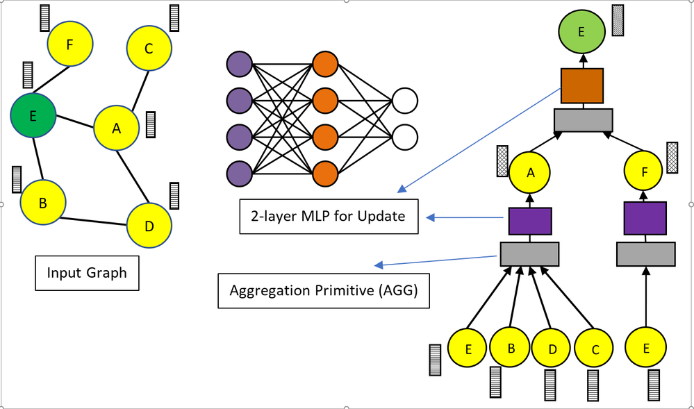
There are two broad flavors of GNN training – full-batch training and mini-batch training via sampling techniques. Depending on the type of graph data, a data scientist may choose either flavor for their application. In full-batch training, all nodes in the training dataset participate in the computation in every iteration; because each vertex is associated with a dense feature vector, full-batch training on large graphs requires a large amount of memory to store both the embeddings and their gradients. On the other hand, mini-batch training selects a set of vertices and associated sampled neighborhoods from the training dataset every iteration; if the vertex set size is small and the extent of the sampled neighborhood around each vertex is limited, then mini-batch training presents lower memory capacity requirements. In either flavor, the two key primitives involved in the computation are (i) Aggregation and (ii) Update. Figure 1 pictorially represents the entire process of GNN training using these two primitives. We now describe these two primitives.

Figure 1. Aggregation and Update in GNN Training for vertex E

Aggregation Primitive

Let G (V, E) be the input graph with vertices V and edges E and let Fv and Fe be the associated vertex and edge features, respectively. The sizes of Fv and Fe are |V| x dand |E| x d respectively, where 𝑑 is the feature-vector size. We can represent Aggregation as a tuple (Fv, Fe, ⊗, ⊕, Fo), where ⊗ and ⊕ are element-wise operators on Fv or Fe (or a combination thereof) and Fo is the output feature associated with a vertex or edge. ⊗ can be an element-wise binary or unary operator. In binary form, it operates on a pair of inputs; valid pairs are (Fv, Fv) and (Fv, Fe), in an appropriate order. The operator ⊕ performs element-wise reduction on the result of the binary operation to the final output. Mathematically, if AGG represents the Aggregation operation, then

If one of the operands, say y does not exist, then ⊗ becomes a unary operator: it reduces each instance of operand x (using the reduction operator ) into the final output feature-vector z. In Figure 1, the grey-colored boxes in each layer represent AGG. Going from bottom to top, AGG aggregates features associated with vertices B, C, D, and E, respectively, in the first layer and those associated with A and F, respectively in the second layer. We discuss the performance implications of the Aggregation operator in some detail later in this article.

Update Primitive

The Update primitive is typically an MLP consisting of a Linear operator (e.g., torch.nn.Linear) followed by one or more element-wise operators (e.g., Rectified Linear Unit (ReLU), DropOut, etc.). The Linear operator contains learnable parameters (i.e., weights and biases) that together constitute the GNN model. As shown in Figure 1, the model weights are represented as connections between the purple- and brown-colored neurons, as well as between the brown- and white-colored neurons in the example 2-layer neural network. Thus, the Update primitive produces an updated set of vertex embeddings by filtering them through model parameters after the Aggregation primitive aggregates initial vertex embeddings.

GNN Training Process

End-to-end GNN training consists of recursively applying Aggregation and Update primitives in sequence over several hops. Typical GNN topologies consist of 2-3 hops, although there are variants that contain 10s or 100s of hops. The overall training process is as follows: starting with a set of initial embeddings on each vertex, the Forward pass applies AGG followed by Update for each hop (also called layer) in the GNN. Subsequently, the loss layer (e.g., Cross-Entropy loss) computes the error with respect to a target vector (e.g., node labels) and backpropagates the error through the GNN in reverse order. Each MLP computes the error gradients with respect to the model parameters. At the end of the Backward pass, the gradient-descent optimizer (e.g., Adam) updates model parameters, completing one iteration of training. This process repeats for a specified number of iterations or until a convergence criterion is reached.

GNN training: Optimizations for Intel® Xeon®

The well-known Deep Graph Library (DGL) implements graph data-structures (e.g., Adjacency Matrix) in standard Coordinate list (COO), Compressed Sparse Row (CSR), and Compressed Sparse Column (CSC) formats and provides a rich set of abstractions along with built-in functions to implement variants of the Aggregation primitive. It supports PyTorch among other neural network frameworks and uses its autograd functionality to implement automatic differentiation. It implements the core graph manipulation and Aggregation primitive functionality in C++.

DGL represents initial vertex features as a PyTorch Tensor object, enabling both AGG operations and various neural network operations on them. Figure 1 and the above discussion implies that representing the graph as an adjacency matrix and vertex features as a dense PyTorch Tensor object will result in the following sequence of operations for the AGG primitive:

1. Irregular memory accesses to read or gather feature-vectors of each vertex and its neighbors from memory as indicated by source vertex indices
2. Apply ⊗ on each Fv, (Fv, Fv), or (Fv, Fe) tuple to perform unary or binary operations, respectively and
3. Apply ⊕ to reduce each source vertex or edge feature-vector, and
4. Irregular memory accesses to write or scatter the resulting feature-vector the Tensor object in memory as indicated by destination vertex indices in the adjacency matrix.

Operations 2 and 3 above are compute-bound and can be accelerated using multi-core support, caches and SIMD units per core in Intel® Xeon® CPUs; for the former, we employ dynamic thread-scheduling using the OpenMP library and for the latter, we employ the Tensor Processing Primitives (TPP) [1] in the LIBXSMM library [2] to generate optimal SIMD code. However, operations 1 and 4 are memory-bound operations whose performance may be limited by both memory latency and the achievable memory bandwidth utilization to access vertex or edge feature vectors. To reduce memory latency and improve memory bandwidth utilization, we apply cache blocking on the source vertex feature-vector tensor, potentially accessing the whole destination vertex feature-vector tensor repeatedly. Details of this technique and associated algorithm are described in [3].

Optimizing the MLP primitive consists of blocking and transforming the layout of the model parameters to take advantage of caches and register files to maximally reuse weights, and fusing element-wise operators such as ReLU and Dropout along with the matrix-matrix-multiply operation of the Linear layer. Again, we use LIBXSMM TPP-based JITed code for all these operators. Further, we use OpenMP to take advantage of multiple cores in each Intel® Xeon® socket to parallelize these MLP computations across the batch dimension.

GraphSAGE Performance on Intel® Xeon®

The GraphSAGE model is either a 2-hop or 3-hop GNN depending on the dataset. To evaluate the performance of our optimizations, we implemented them in DGL and executed an application using the GraphSAGE model on 3 different datasets – Reddit, OGBN-Products, and Proteins. Table 1 shows the sizes of the graphs in these datasets.

Table 1. Dataset specifications

Full-batch training on a single node

Our analysis of the GraphSAGE workload on an Intel® Xeon® 8360Y CPU with 36-cores per socket indicates that AGG execution time determines the overall performance of this workload; the MLP consumes a very small portion of overall execution time. Therefore, our optimizations to AGG are critical to the performance improvement of this workload on Xeon. These optimizations are now part of the master branch in DGL Github repository (https://github.com/dmlc/dgl). In the charts below, we define Baseline performance as that obtained without turning on our optimizations available in DGL (USE_LIBXSMM=OFF).

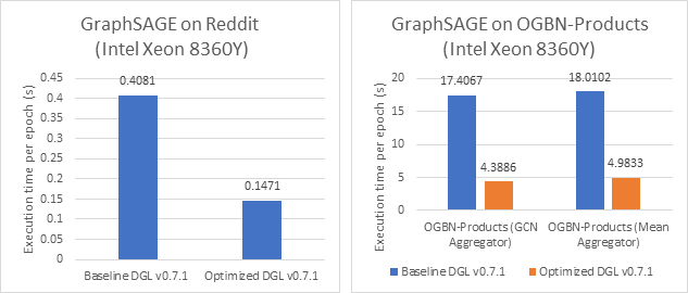
Figure 2. Performance of full-batch training (Reddit and OGBN-Products)

Figure 2 shows the performance of GraphSAGE for the Reddit and OGBN-Products datasets while executing on a single socket of the Xeon CPU. We clearly observe that our optimizations to AGG result in approximately 2.77x speed-up for Reddit, 3.96x on OGBN-Products when using the GCN Aggregator operation, and 3.66x on OGBN-Products when using the Mean Aggregator operation.

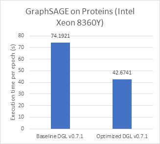
The Proteins dataset is significantly large (167 GB); therefore, we employ both the sockets on a dual-socket Intel Xeon 8380Y for a total of 72-cores and 256 GB of memory. Figure 3 shows the performance of GraphSAGE on the Proteins dataset. Again, we observe that our AGG-optimized code executes approximately 1.74x faster than the baseline code.

Figure 3. Performance of full-batch training (Proteins)

Minibatch training on a single node

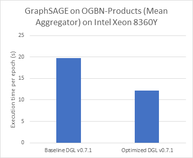
In contrast to full-batch training, we observe that the minibatch training performance of this workload depends on both AGG and MLP, approximately equally. Therefore, our optimizations to both these primitives are applicable. We are preparing to upstream these optimizations to DGL master branch. Again, in the chart below our definition of Baseline performance is that obtained without turning on our optimizations available in DGL (USE_LIBXSMM=OFF). Figure 4 shows that our optimized code achieves approximately 1.62x speed-up over the baseline implementation.

Figure 4. Performance of minibatch training (OGBN-Products)

Conclusions and Ongoing Work

Graph Neural Networks are an important new class of AI workloads. This article demonstrates the ability of modern Intel Xeon processors to deliver impressive performance for this class of workloads when the underlying software primitives are well-optimized to take advantage of available architectural features. We continue to focus on this important workload – our paper on distributed GNN training [3] described an approach to scale GNN performance from a single node to multiple nodes. We are refining that approach and attempting to cover other classes of GNNs, beyond GraphSAGE in our optimization efforts.

References

1. Tensor processing primitives: a programming abstraction for efficiency and portability in deep learning workloads, E. Georganas et al., In Proc. Supercomputing 2021 (SC’21)
2. LIBXSMM: https://github.com/libxsmm/libxsmm
3. DistGNN: scalable distributed training for large-scale graph neural networks, V. Md et al., In Proc. Supercomputing 2021 (SC ’21)