Interesting Observations

[JohnNichols]

I have had a lot of fun and some heart ache playing with the MKL Library and the PARDISO solver.

The PARDISO solver is very fast.  The problem I am solving is the hydraulic network problem, in this case using the Gradient Method. The PARDISO solver gives a much better first estimate of the solution vector, which can be measured using the error on the sum of the hydraulic heads. It's first pass gives a 4 fold better estimate than the other solvers (all that I have tried).

But the solver then converges very slowly to the "best estimate" of the answer, taking 8000 iterations to do what the others do in 20. So the fact that the iterations are fast, is lost in the slow convergence.

I have played with passing the A array into the PARDISO solver in different formats, both the sparse and the dense matrix, it makes no difference.  Rum really. I look step by step at the solution vector, and it is a long way from the other inversion solution vector even on the first iteration for the fully dense solvers.

Interestingly if I run as a PHASE 33 - I get errors, but it works, if I use 13 - it also works slowly, but I do not get the errors.

It does solve, but it is not faster in the end than the other solvers, interesting really.

Question: Should I try another MKL solver?

JMN

[JohnNichols]

Dear mecej4:

Thank you for the code. I will implement the mag check code inside MagniCSR.

I enclose the program with a drawing routine added to draw the network map as a DXF file.  It is relatively easy given code I already have to write this type of DXF generator program. I did it between tutorials today so it is old and rough, the original was written in 88.  I can also add a routine to draw the map as bitmaps but that is a bit harder. This new stuff will allow me to plot out a Richmond plan so I can see where the catchments are.

I would like to add a contouring routine to show the residual heads on the plan in addition to the model data.  I have some code, but it is very old and need s fair amount of work.

Yes, it is nice to allow the modellers to name the nodes, although as a long time engineering modeller I like plain numbers.  Rossman moved from plain numbers to the node names in going from the 91 to the 98 model, but looking inside EPANET he maintains the model with just numbers and simply adds an ID, but when he prints out the .INP file he discards the model numbers and assumes you can reassemble the model from the ID's. An extra column with the integer model numbers attached to the ID's would not hurt anyone.  The problem with this 98 technique is the range of alpha groups possible if we consider a small  limit of 6 character groups, , this is a 37 to the sixth power, which is 2.56 billion number combinations.  The Richmond model uses upto 11 apha characters. The other critical element is the water zone the node lies in,  the Richmond model appears to cover a County type area in Yorkshire, so there would appear to be reservoirs scattered on a set of hills as you move away from the source point, called reservoir in the RICH model. The system is connected with pumps basically pumping in a linear tree fashion away from the reservoir.  I am not sure, but I would guess each little town, city takes its water from a single reservoir or maybe two in the system. So we have a fairly stable demand that will be well known at the hourly point throughout the year, so why build a huge transport model with a small catchment models added on, one could just as easily model the trunk alone. A lot simpler and much easier to understand in the long run.  Of course mine is not to reason why, but sometimes one wonders.  I actually think your idea of modifying EPANET is better, the C code can be added to the output routine to save a model with the integer numbers and the ID's.  Rossman does ot use the ID's as an index, it is merely a name.

I am not sure if you have AutoCAD so I have added in plots of the filem file. 

JMN

[JohnNichols]

I fixed the node in TAM model, on the original drawing it had been moved to the wrong layer and so the DXF read routine missed it completely.  Node 3002 should be 3004.  The southern part of the town has One Tree Hill, which has a set of interconnected reservoirs, but the town allowed  people to move to far up the hill and they needed a high level system, based on a pumping station - bad idea of course as no power no water. The set of reservoirs in this area is quite complex, so I have pulled out a small part at the top of the hill and I have got this working so that I can remember how the systems work.  I can also draw it at large scale so you can see the node numbers.  I pulled out the first 100 nodes, it required 5 tanks to make it work and not crash.  I have included a routine that checks which tank a network component is connected and then assigns a zone number based on the tank number.  There are three pumping stations on this system as well so I will put them in and get them working before I start adding bulk nodes.  This network has quite a few pipes that hang off like leaves, with zero demand on these pipes the program gets a bit upset and iterates to the limit. Each pipe that is an end pipe appears to need a small base flow to ensure the program does not go into ga-ga land.

I will incorporate your check program into MagniCSR - it works a treat - thanks. I enclose the latest iteration. It needs a lot of cleaning, but at least it works nicely now.  I would not have made it with out your help - many  thanks again.

Have a nice weekend. 

I also want to put in a limit, so one can say - only do this zone etc. 

JMN

[JohnNichols]

I was looking for a routine that would contour 3D data, it is a pain to do it in other programs. CONREC is good for rectilinear data, but the water supply problem has scattered data.

AKIMA developed an algorithm back in the 80's and there are several implementations, but the ones in the TOMS library do not play nice with IFORT - the FORTRAN is to old and the changes are extensive.

I stumbled across the R package for this routine and it is written in Fortran in about 2005.  It is not perfect, but it works and it was not hard to write a program to test the data input format and try the program.  The output is a rectilinear gird with the estimated data heights. I enclose the code, it is freely available in the R package as source code, so one presumes it is ok to use it elsewhere, there are multiple published versions in public locations.  It should work with CONREC to give me nice BITMAPS of the contours of the water supply plans.

526 is the number for the routine in the TOMS library. I kept the number.

JMN

[mecej4]

MKL has an Akima routine, which you may want to peruse for suitability. There are a couple of 1-D Akima Matlab packages at the Mathworks File Exchange. There are 1-D and 2-D Akima interpolation schemes. I presume that you want the 2-D version, since TOMS 526 is for 2-D.

I don't know what you mean by "does not play nice". Of course, TOMS 526 was published when F77 was just being born, so you should expect it to be mostly Fortran IV. I just tried the 526.gz file and the example ran fine with IFort. You probably tried with run time checks -- that will not do with such old code, which follows the old convention of declaring dummy array arguments with dimension (1) where we would now write dimension (*). That '1' is just syntactic sugar.

[JohnNichols]

Dear mecej4:

I did get 526 working with VS 2013, but it took a while and then when I tried to pair it with 626 to have a driver program it was reaching the stage of not being worth the effort, and I stumbled across the AKIMA stuff in the R library. This R stuff has been fixed by the original authors and a few others for Fortran 2005, so I grabbed it, it did not take long to get it in a form that will fit nicely into Magni.  I was not looking forward to updating all of the older code, luckily I did not have to , thank god for the NET.

I had read quite a bit that Steve had written on the syntactic sugar problem. I should have tried IFORT, but I am so fond of the VS Studio IDE that I tend to use it for everything, which is a problem.  I should have switched off the interface option, but just as I read that in one of Stevel's post I found the R version.

Adding the drawing routine to MAGNI has been worth the effort, in the next post I will include the recent output.

JMN

[JohnNichols]

[JohnNichols]

[JohnNichols]

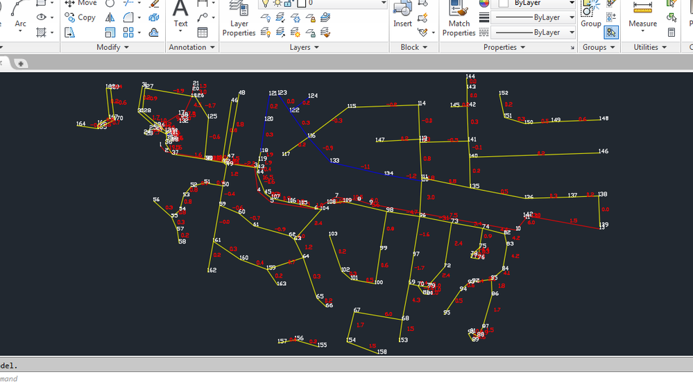
The first picture shows the area around One Tree Hill in Tamworth. The picture shows the pipes, node numbers, and flows in L/s. I have the heads turned off for the moment.   The error routines now trap the obvious errors, the one I need to work out a solution for is the lack of a reservoir on an area of pipe. I am thinking that I add a fake reservoir that connects to any node - pipe - node set not connected to the network. At the moment an error message pops up and says the network segment is isolated.

It is interesting to look at the order of entry of the nodes and pipes, there is a scattering pattern.

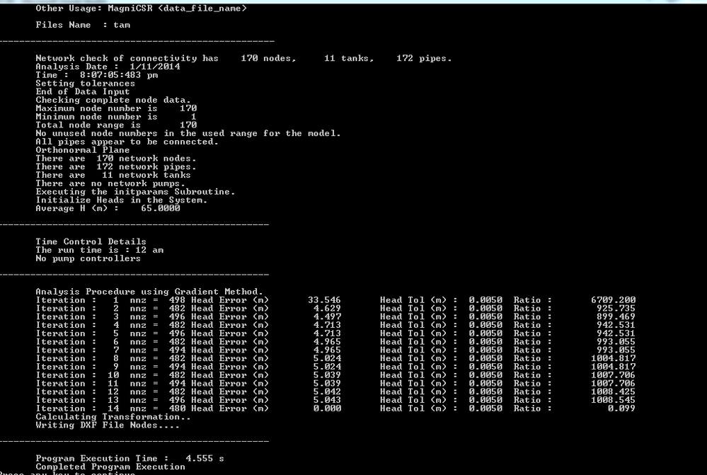
The second pictures shows the iteration data for the previous picture. The head error pattern is interesting, it could be related to a pipe with zero flow. Zero flows in terminal pipes cause some angst to the program.   I am at 170 nodes so it getting to a reasonable size.

JMN

[JohnNichols]

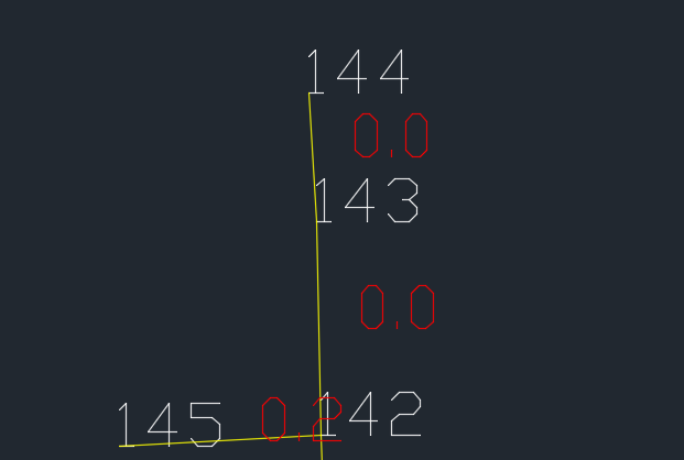
I put in a write statement to watch the F(I) error in the output. Node 143 showed a large error > 5m for 10 iterations, whilst all of the other nodes were low. Node 144 was connected only to 143,  and 143 was connected to 142.

Both nodes had zero demand.  Changing the demands settled down the F(I) values quickly, still took 11 iterations, but by iteration 2 all the levels were low.  There needs to be a demand on all terminal pipes in the graph. Interesting to play with it and see what is an acceptable minimum. Also provides another error or warning condition to check for.

[JohnNichols]

Dear mecej4:

So the change in the NNZ count is the changes in the number of entries in the sparse array, so some entries are filling in on some iterations, interesting to see how it bumps around. If NNZ is 3 times the number of nodes, then a 100,000 element model should be possible - not pleasant but possible.

The drawing routine is the slowest routine by a long shot now, almost 3 seconds for the 170 nodes and 178 pipes.  But being able to see the output is great.

Thanks for all the help.

JMN

[mecej4]

You appear to be surging ahead with an analysis package that is approaching release quality. I'd appreciate access to the fixed up TAM.INP that you used for the screenshot in #70.

I do not have Autocad, nor have I ever used it. All the drafting that I have ever done was on big drawing boards with T-squares, set-squares, etc.

[JohnNichols]

Dear mecej4:

I enclose the latest iteration, the program is sweet, I would never have made it without your help, thanks so much.

I have the contouring package sorted out, I always draw first in DXF format because it is so easy to debug, I have been using that technique since the mid 80's. In the olden days only the VEDIT editor would open the megabyte DXF files we created for the sewer systems.  It was an obscure program done by a funky team from the northern part of the USA, but they are nice people, It used to run the FORTRAN Microsoft compiler inside the program and give you the output in a edit window.  it had a great language built in.  It was really great.  It is nicer in the end than the others. Still use the latest version.

I will go back and add bit map images for the output, this is just a little bit more painful than DXF. I have a drawing board in my office, still use it.

The file is called TAM.INP. I am going to sort out the check valves, reservoirs and the node names before I try to expand this file beyond this size.  It is also a nice size to test the program busting features like double pipes between nodes.  I know an engineer in Tamworth who used to work for me so I will see if I can get the contours.

We should be able to read the EPANET binary file straight into Fortran correct?  If so we can I think overcome the lack of numbered order lost in Rossman's ASCII files.  I still prefer his 91 to 98 program.

Solid works gives away a DXF viewing program.  I am just trying it. it works a treat and it is free. I just looked at the TAM drawing. There are a number of advantages in program development of having a DXF plot instead of a bitmap plot.

[JohnNichols]

Dear mecej4:

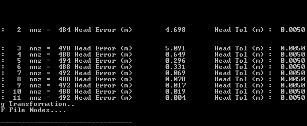
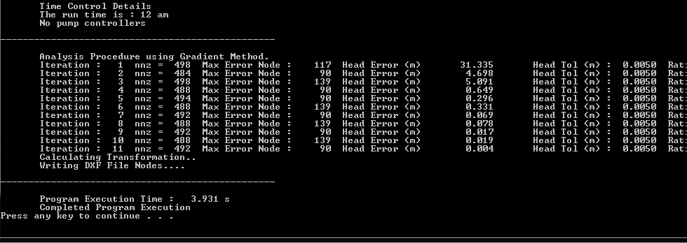
I added a brief line to keep track of the Node Number with the highest head error, the attached capture shows the revised output. It showed one of the zero flow nodes for TAM.  This makes it easy to go and look for mistakes.